After Einstein and Bose predicted, at the beginning of the 20th century the
existence of a new state of matter it took about 100 years that the
first so called, Bose-Einstein-Condensate (from now on BEC) was realized experimentally.
The BEC is a special state of Bosons, which can be derived from the Bose-Einstein-Statistics.
The State of BEC is reached at very low tempratures, where the majority of particles occupy
the ground state of the system. All particles in the condensate are delocalized
and each particle has the same probability density. We can consider
the whole BEC as a one quantum state particle which yields to the great
possibility that we can describe it as one wave function. Now we can observe
quantum effects on a macroscopic scale.
In the first prediction of the BEC it was considered as an ideal gas, which
isn't suffcient description, because of the missing interactions between the
particules. A theory of interaction in a BEC was given by
Gross and Pitaevskii and yielded to a succesful description of the
superfluid $He^4$.
The Gross-Pitaevskii Equation can be seen as a Schroedinger-equation
with an additinonal term for the interaction in the condensate where
$$g=\frac{4\pi\hbar^2a}{m}$$
($a$ the atomic scattering length and $m$ the mass).
\begin{equation}
i\hbar \partial_t \psi = \left( -\frac{\hbar^2}{2m} \nabla^2+V_{ext}+g|\psi|^2
\right)
\psi
\end{equation}
The subject of this work is to understand the effect of chaos on Josephson like oscillations.
Josephson oscillations were first created with superconductors seperated by a small tunneling barrier.
The oscillations are the result of Cooper pairs who tunnel the barrier. Cooperpairs are
two electrons thus Fermions with opposite spin who behave together like Bosons.
The effects can be described by by two seperated wavefunctions for each superconductor
and a superposition at the barrier. From the GPE one can now derive.
\begin{equation}
i\hbar \frac{\partial\Psi_{1,2}}{\partial t}=E_{1,2}\Psi_{1,2}+K\Psi_{1,2}
\end{equation}
In our model we will condsider a BEC in a nonsymetric double well potential.
This is a generalized form of the previously mentioned model, because of the
non-symmetric potentials.
Model without Chaos effects
We consider a BEC in a non-symetric double-well-potential.
The system is described by the GPE. With the ansatz
$$\Phi =
\psi_1(t)\Phi_1(t)+\psi_2(t)\Phi_2(t)$$.
and the property $$\int d\vec{r}\, \Phi_i \, \Phi_j = \delta_{ij}$$
we can derive two coupled differential Equations for $\psi_1$ and $ \psi_2$ .
The ansatz is so far valid for our problem, because we consider the condensate
as weakly linked, that means that we have a superposition of the solutions for
each well independently. This is the same assumption as mentioned before for
the Jospehson effect. The solutions for each well are called
$\Phi_i$.
$$
i\hbar \partial_t \psi_1 = (E_1^0+U_1N_1)\psi_1 - k\psi_2\\
$$
$$
i\hbar \partial_t \psi_2 = (E_2^0+U_2N_2)\psi_2 - k\psi_1
$$
The constant $E_i^0$ is the energy in each well depending on the
shape of our double-well-potential. $U_i$ is the interaction term inbetween the
particules and $K$ describes the coupling between the two wells thus the
tunneling effect. These values can be calculated by the integration over the
eigenfunction of the two separeted wells or for $K$ over the overlap of the
eigenfuntions.
\begin{align}
E_i^0 = \int d\vec{r} \left[ -\frac{\hbar^2}{2m}\Delta\Phi_i + V_{ext} \Phi_i
\right]
\end{align}
\begin{align}
K = -\int d\vec{r} \left[ \frac{\hbar^2}{2m}\nabla\Phi_1\nabla\Phi_2 +
V_{ext}\Phi_1\Phi_2 \right]
\end{align}
\begin{align}
U_i= g \int |\Phi_i|^4 d\vec{r}
\end{align}
According to the Mandelung Transformation the complex variable $\psi_i$ has the general form
$\phi_{1,2} = \sqrt{N_{1,2}}e^{i\theta_{1,2}}$, where $N_i$ is the number of
patricules in a well and $\theta_i$ a abstract phase of the system, with this transformation the GPE is
now interpretable. The ansatz yields to our new system depending on $\phi$ and $z$ .
Therefore we have used the substitions $\phi = \theta_2 -\theta_1$
$0 < z = \frac{N_1-N_2}{N_t} < 1 $ and
\begin{equation}
\Delta E = E_1^0-E_2^0 +\frac{N(U_1+U_2)}{2} \qquad\Lambda =
\frac{U_1+U_2}{2}N
\end{equation}.
You can see $\Delta E$ describes now the symmetry between the two wells.
The equations for $z$ and $\phi$ can be derived from a Hamiltonian with the
conjugate variables $z$ and $\phi$. The Hamiltonian has the form
\begin{equation}
H(\phi,z)=\frac{\Lambda}{2\hbar}z^2+\frac{\Delta
E}{\hbar}z-\frac{2K}{\hbar}\sqrt{1-z^2}\cos(\phi)
\end{equation}.
To understand chaos effects in this nonlinear coupled equations it is necessariy
to figure out the features of the system without chaotical behavior. This
will help us to seperate the chaos phenomena from the ones which comes from the
one which are naturally in the model.
\begin{equation}
\frac{\partial H}{\partial z} = \dot{\phi} =
\left(\frac{2K}{\hbar\sqrt{1-z^2}}\cos\phi +\frac{\Lambda}{\hbar}\right)z +\frac{\Delta E}{\hbar}
\end{equation}
\begin{equation}
\frac{-\partial H}{\partial \phi}= \dot{z} = -\frac{2K}{\hbar}
\sqrt{1-z^2}\sin\phi
\end{equation}
Macroscopic quantum self trapping (MQST)
At first we are going to look at the model without the term $\frac{\Delta E}{\hbar}$ with is depending
on the interaction between the particules and the shape of the wells and is 0 if the two wells are symmetric.
We introduce a $k = \frac{K}{\Lambda}$. Depening on the choice of the parameter k we obtain qualitative different
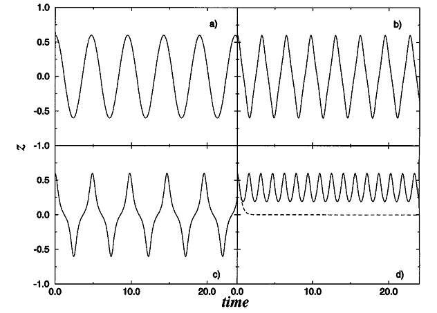
types of oscillations of the imbalance of the condensate (see FIG. 1).
For a great k we can observe sinusoidal oscillations around 0 with a smaller k they get more and more anharmonic
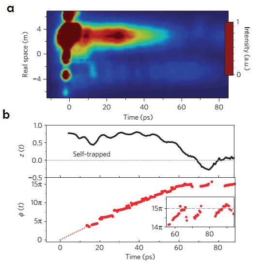
and lead into mqst. In the mqst the condensate oscillates not around 0 as a classical pendulum would do instead
it is oscillating around an imbalance. This phenomena was, for instance, observed by a group a researchers in 2013.
The condensate was self-trapped for about 60 ps while the phase was growning linearly (FIG.2)
FIG.1 Fractional population imbalance $z(t)$ versus rescaled time, with initial conditions $z(0) = 0,6$, phase difference
$\phi(0) = 0$, and $\Lambda \sim \frac{1}{k} =1$ (a),$\Lambda \sim \frac{1}{k} =8$ (b), $\Lambda \sim \frac{1}{k}=9.99$, $\Lambda \sim \frac{1}{k}=10$ (dashed line, d), $\Lambda\sim \frac{1}{k}=11$(solid line, d)
(from 2013, M. Abbarchi, A. Amo, V. G. Sala,D. D. Solnyshkov, H. Flayac, L. Ferrier, I. Sagnes, E. Galopin, A. Lemaître, G. Malpuech and J. Bloch
Macroscopic quantum self-trapping and Josephson oscillations of exciton polaritons ) FIG.2 Measured dynamics of the emitted intensity.,a Time evolution of the
population imbalance and phase difference.,b
(from 1997, Smerzi, A. and Fantoni, S. and Giovanazzi, S. and Shenoy, S. R.
Quantum Coherent Atomic Tunneling between Two Trapped Bose-Einstein Condensates)
Further dynamics of the condensate and fixpoints (work in progress)
For further understanding of the model we try to find the fixpoints and examinate their stability.
We have to solve the follwing equations to find the fixpoints, which gives us the following 7 different fixpoints.
\begin{equation}
0 \overset{!}{=} \dot{\phi}
=z + kz\frac{\cos\phi }{\sqrt{1-z^2}}
\end{equation}
\begin{equation}
0 \overset{!}{=} \dot{z} = -
\sqrt{1-z^2}\sin\phi
\end{equation}
$z = \pm \sqrt{1 - k^2}$
$ \phi = \pm \pi$
$z = \mp \sqrt{1 - k^2}$
$ \phi = \pm \pi$
$z = 0 $
$ \phi = \pm \pi$
$z = 0 $
$ \phi =0 $
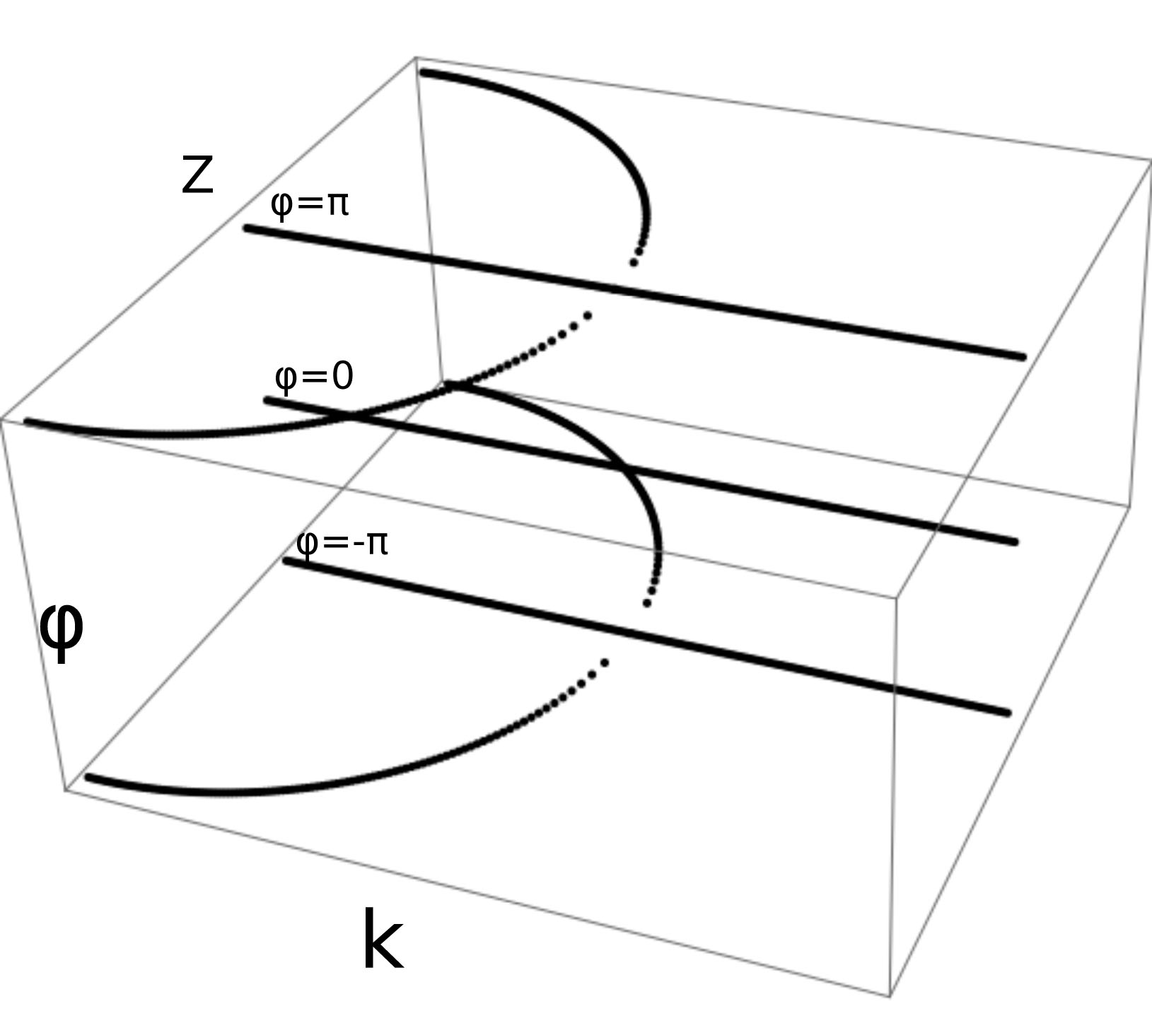
FIG.3 Bifurcation Diagram of the model without disturbation. k was choosen from 0 to 2 in the dotted line is no information
about the stablity of the branch.
One can see the symentric behavoir of the system at $\phi = \pm \pi$ in the Bifurcation diagram.
The fixpoints which depend on $k$ get imaginary for $k>0$ what means they don't exist in reality. The point
of bifurcation is $k=1$. The bifurcation is depending on strength of
the coupling and the interaction inbetween the particules. We can say, that for a bigger coupling we have only 3 Fixpoints and for bigger
interaction in the condensate we have 7 Fixpoints.
Model with Chaos effects
The next step will be to add chaos features to the model and try to understand the
behavior of the system.