Calibration of the speed of the vein
Introduction
The hydraulic vein delivers a flow which speed is based on the frequency of the motor of the vein, measured in Hertz. In order to convert from Hertz to Meters per Second, a calibration of the vein is mandatory.
Two methods are available, the first one is based on a dye dropped in the vein and the other one is based on Partcle Image Velocimetry.
- Dye Calibration -
Uncertainties
- Experimental : the motor provides a motion which velocity is determined by a frequency. However, this frequency is delivered with a precision of 0.01 Hz.
- Experimental : the grid we use to measure the flow isn’t perfectly aligned with the bottom of vein. Therefore, a mistake appears and is equal to the sinus of the angle between the bottom of the vein and the horizontal line of the grid.
- Instrumental : the caracteristic length of the grid is set in millimeters. Therefore, we have an uncertainty of -/+ 1 mm.
- Statistical : the image processing creates a statistical uncertainty. Indeed, the user has to set the moment the colorant passes the line of the grid. This moment is estimated within a range of a few images.
Protocol
- Turn on the motor set on the frequency you desire to calibrate, wait a few instants for the flow to become stationnary.
- Pour the dye into the vein. Depending on the frequency, the colorant should be poured whether at the separation of the vein or just before the entry of the observation field.
- Wait for the dye to reach the field of the camera and launch the acquisition. Stop the acquisition when the colorant reaches the end of 1 section of the grid (or the 5 sections, for more precise results).
- Process the data with ImageJ.
Constraints and Advantages
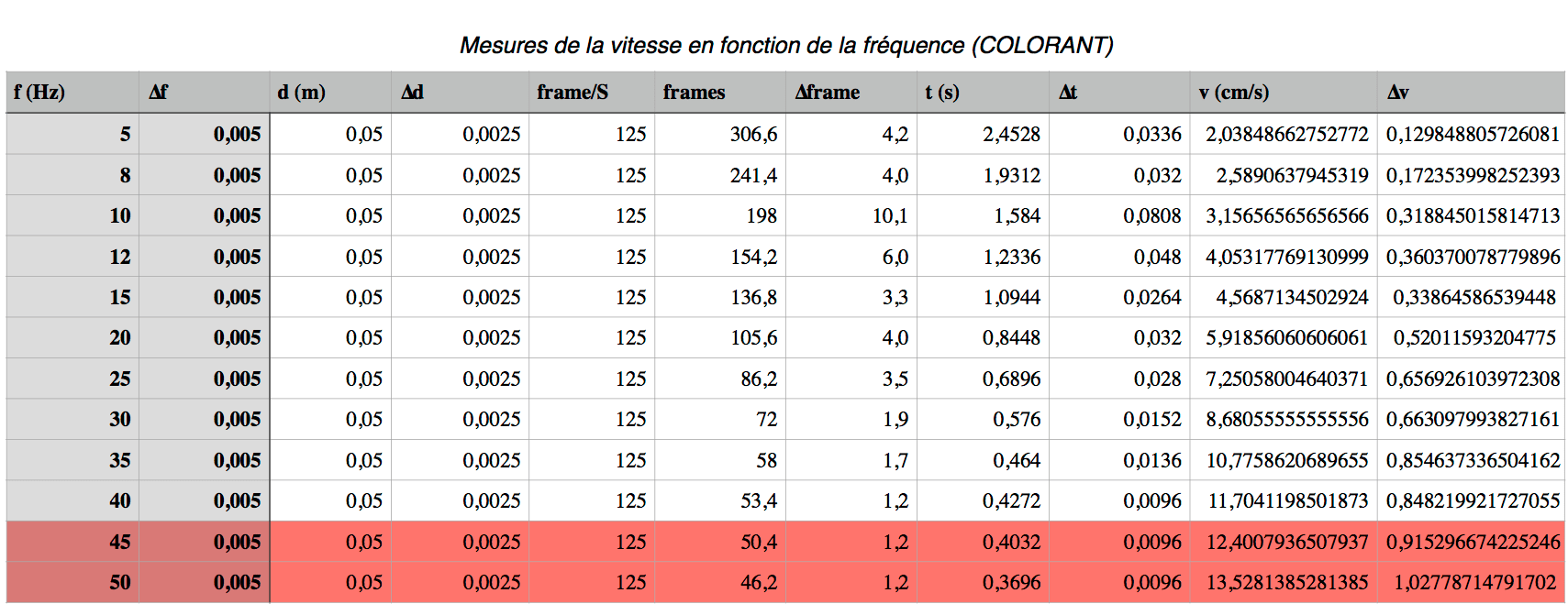
- Colorant dispersion inside the flow: When the dye liquid is poured into the vein, it doesn’t spread evenly in every direction. Therefore, it is hard to distinguish the exact moment when the colorant crosses our grid of measurement.
- Framerate : 125 frames/sec. We set the camera with a higher frame rate than the PIV. Indeed, we set up a grid on the observation glass inside the vein and it is not necessary to shoot 10 seconds video. It is more likely to be set aroung 4 seconds since we activate the shooting by looking directly at the dye and we stop it when we wish to.
- Tools of precision: Our grid has 5 divisions which measure 5 cm each. By doing so, it is possible to measure the time, the colorant crosses the grid and we can evaluate the inaccuracy by using a statistical method.
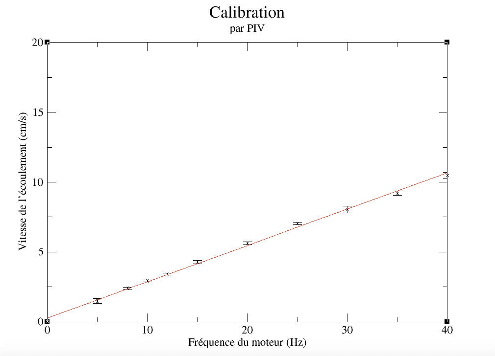
Results
Conclusion
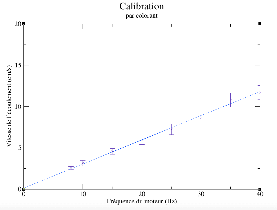
The velocity of the flow inside the vein is linear. Therefore the theory is confirmed. By looking at the array containing all the results we have, we can understand a few things.- The number of frames is decreasing as long as the frequency delivered by the motor increases. Therefore, the flow speed is increasing with the frequency as the engine. The graphic is thereby empirically true.
- Δt diminishes with the frequency which allow us to theorize that the speed of the flow decreases.
-
According the formula,
V(d,t)= d/t
We have :
Δv/v=|Δt/t|+|Δd/d|
Which stands true since all the deltas are diminishing or remain constant.
- Particle Image Velocimetry Calibration -
Uncertainties
- Experimental : The motor provides a motion which speed is set with a frequency. However, the frequency is delivered with a precision of 0.01 Hz.
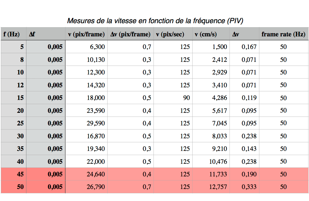
- Mesure : The length of the camera field : d = 5 cm ± 1 mm. d=210 ±3 px.
- Experimental: Since we didn’t have the protection required to use a high intensity laser, an error of precision remains.
- Experimental : The angle on which the laser layer is set has an intrinsic error.
Protocol
-
Set a black screen on the glass window of observation to improve the measurement. Throw particles with a small diameter (~µm) into the vein:
- HGS (Hollow Glass Sphere) : 10µm.
- PSP (Polyamid Seeding Particle): 50µm.
- Turn on the motor and set it on the frequency we want to calibrate (between 8Hz and 50Hz). The reason why the experiment isn’t carried under 8Hz frequencies is that due to a short amount of time available for this project, the flow speed wouldn’t have allowed us to fulfill other experiments.
- The video acquisition is then processed on video software such as ImageJ: Selection and reduction of the datas. Since a lot of images have been taken for the video (around 3000 for one shot of 10 seconds), the user must select 1 pictures out of 10 to reduce the size of the video. Compress each picture of the remaining video into an 8bits file. Then operate a data treatment over a software such as Mathlab or Octave to evaluate the correlation over each picture.
- Extract data and convert it from “px/frame” to “cm/s”.
Constraints and Advantages
- Safety googles: This experiment has been conducted without any safety laser googles. Therefore, a high precision of measurement isn’t possible since the laser couldn’t be used with a high intensity.
- Low Frame rate 50 Hz: a frame rate of 50 Hz generates around 1000 images for a 10 seconds long video. Considering the short amount of time we had, shooting videos with a frame rate higher than this would have cost us a tremendous amount of time.
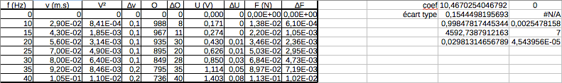
Results
Conclusion
So first of all, we observe that the speed of the flow is proportional to the frequency of the motor inside the vein. Nonetheless, if we approximate our results with a linear equation, a constant at the origin exists. Even thought the method is more precise, the results are less interesting than the colorant method.Force Sensor Calibration
Introduction
Our sensor is able to measure the force applied to the rod, fixed on its base.
Important : the measure does not depend on the position of the object on the rod.
The sensor returns a value between 0 and 1023. As long as the captor measures a voltage from 0 to 5 Volts.
Also, it is necessasry to calibrate the force captor to convert its value in Volts to a value in Newtons.
Uncertainties
- Measure : Using a postal scale surely had an impact on the uncertainties during this experiment. However we managed to have pretty suitable results on our masses by weighing down a bunch of them together at once.
- Experimental : The ∆O used in our uncertainties calculation are obtained with standard deviation. As a matter of fact, we take as force value, a series of mesures done during a short period of time. It gives us an enormous number of points, so we take the average of those series as our final measure and their standard deviation as the uncertainty on this measure.
Protocol
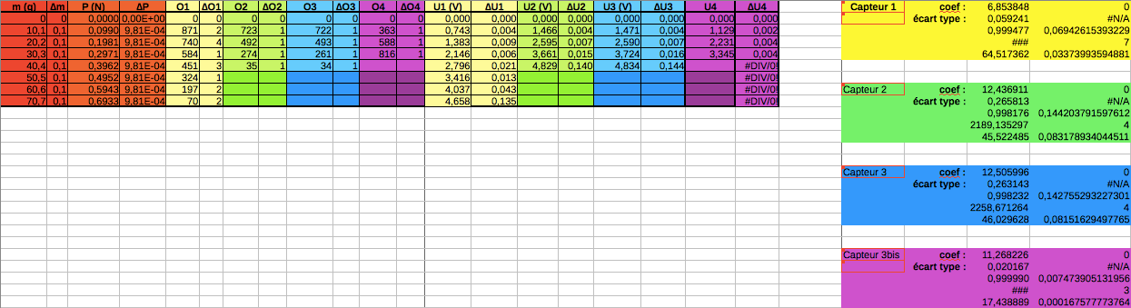
To calibrate our sensor, we are going to use objects with a certain mass which will give us the force applied to these, by using its equivalent of weight in newtons. We decided to calibrate the sensor using the following method:- Weigh down the bolts with a scale to obtain their masses.
- Calculate their weight in Newtons with the formula P = m⋅g where g = 9.81 N/kg.
- Measure the force they apply on the sensor when only subjected to gravity.
- By using a small plastic glass with strings, hang the cup to the sensor horizontally.
- Gather all the data for each bolt and then draw the curve of the force F in function of the tension U by using the software of your choice.
- The slope of the linear approximated straight will give the conversion factor from the circuit output to the the real force applied on the captor.
Constraints and Advantages
- No precise scale: the scale we had at the INLN was the scale used to send letters, not made for our experiments.
Results
Conclusion
Our array is organized as such as it combines the calibration of 4 differents rods from the rod number 1 (O1) to the rod number 4 (O4).- The columns O1 to O4 are the results given by the sensor for different rods.
- The columns from U1 to U4 are the conversion in Volts of the value of O1 to O4 substracted with the value of the 0.
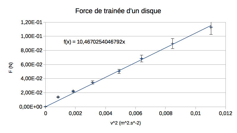
Study of the Drag force applied to a "calibration" diskm; and the fish
Introduction
In this experiment, we will check the theory by looking at the evolution of the force in terms of the squared velocity. To do so, we used a simple disk to calibrate the drag force. We designed the solid with FreeCAD and Simplify3D and then 3D printed it.
Principles and Physics
We take p as the density of the fluid, v the relative speed of the object to the flow, S the area of the cross section and Cx the drag coefficient of the object, therefore we have : F = ½⋅p⋅v²⋅S⋅Cx
Uncertainties
-
Experimental :
on the value of v, obtained during calibration.
-
Experimental :
on the surface S, depending on the accuracy of the 3D printer.
-
Measure :
on the value of F, obtained with standard deviation on our data.
Protocol
-
We place the disk on the sensor rod, making sure the sensor is aligned correctly with the direction of the flow, and the disk faces it.
-
We turn on the vein, starting at 10 Hz (≈ 3cm/s).
-
We then proceed to the acquisition of the force with to the Arduino program.
-
Repeat this process with frequencies between [10Hz , 40Hz] by 5Hz-increments.
Constraints and Advantages
-
Colorant dispersion inside the flow:
When the dye is poured into the vein, it doesn’t spread evenly in every direction. Therefore, it is hard to distinguish the exact moment when the colorant cross our grid of measurement.
-
Frame per second 125 frames/sec: we set the camera with a higher frame rate than the piv. Indeed, we set up a grid on the observation glass inside the vein and it is not necessary to shoot 10 seconds video. It is more likely to be set aroung 4 seconds since we activate the shooting by looking directly at the colorant and we stop it when we desire.
-
Tools of precision:
Our grid has 5 divisions which measure 5 cm each. By doing such, it is possible to measure the time the colorant crosses the grid and we can evaluate the mistake by using a statitical method.
Results
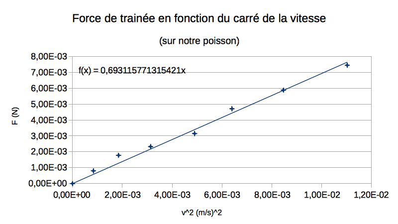
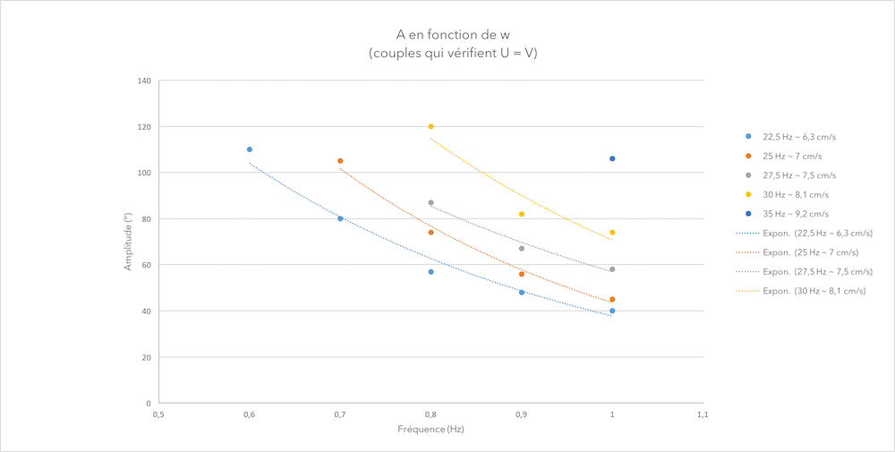
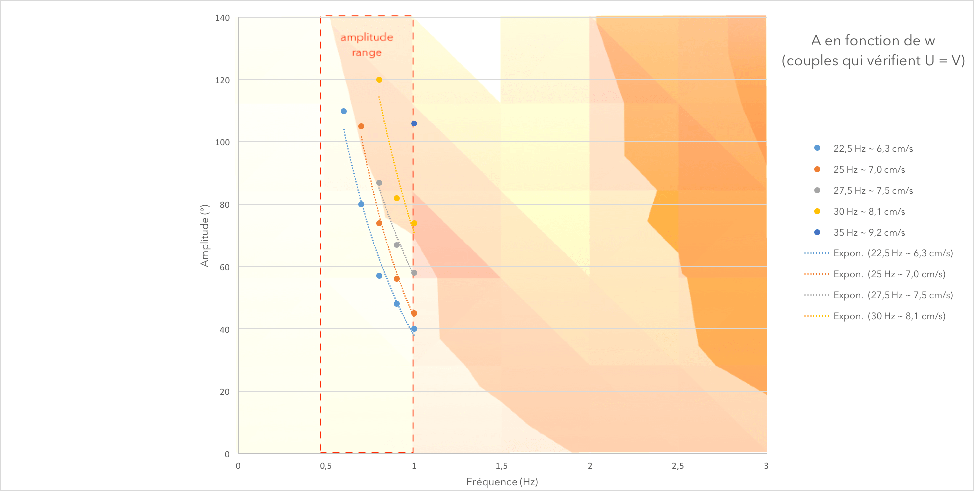
Study of the caracteristic speed U of the Fish
Introduction
This experiment leads us to the core of our project. Indeed, this is the part of the project which allows us to experiment over our supervisor’s theory.
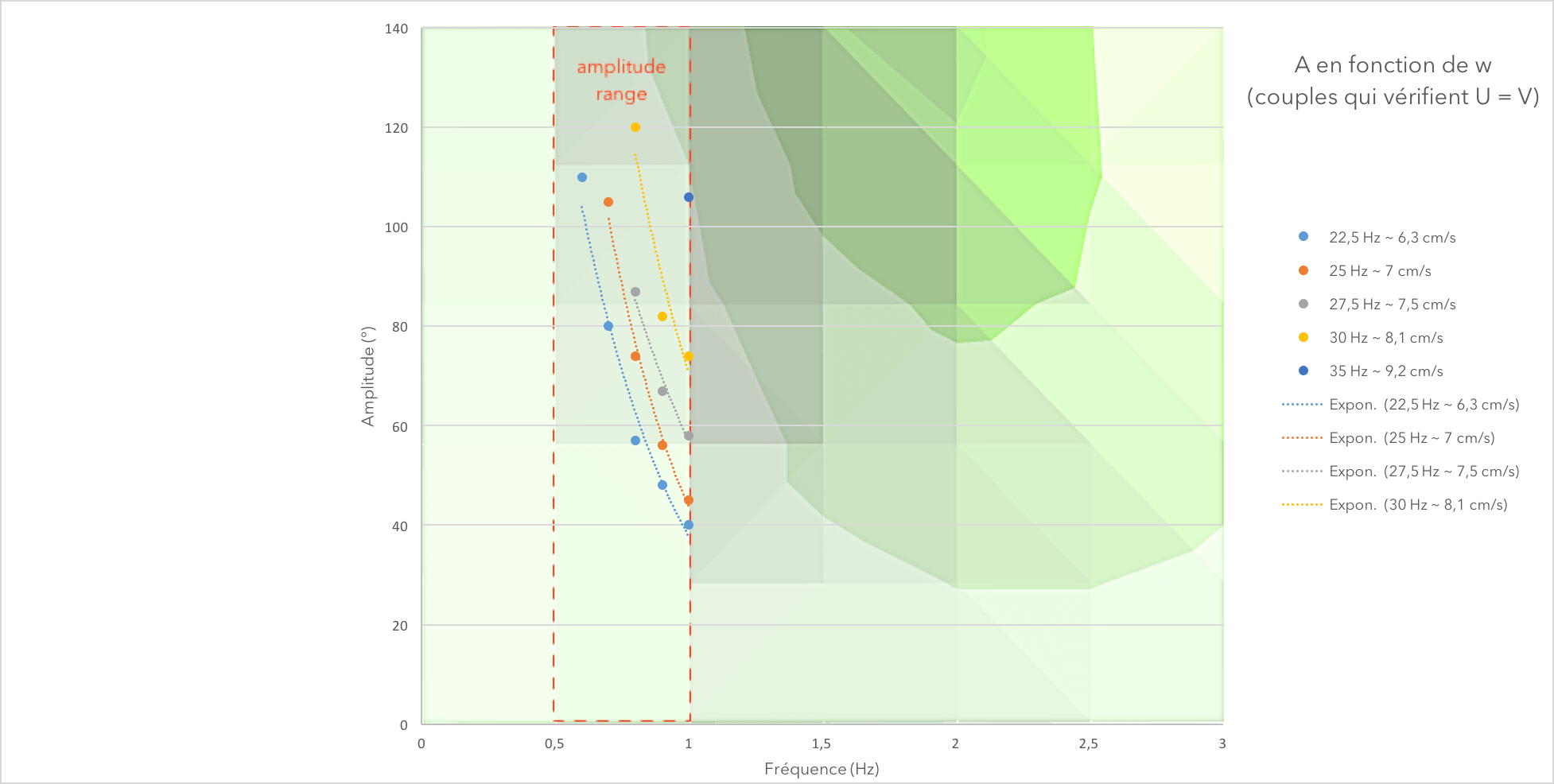
Let U be the caracteristic speed of the fish.
Let A and w be respectively the Amplitude and the Frequency of the motion of the fish's tail.
U ~ A⋅w
Principles and Physics
First of all, the fish prototype is set up inside the vein and attached to the rod. The motor creates a flow which speed, we will name V. If we apply a couple (A,w) to our robot, then it will move with a speed U in the opposite direction of the flow. In theory, if the speed U of our fish matches the speed V of the flow, then in the referential of the vein, the fish will be static and therefore the force applied to the rod will be equal to 0. Finally, by noting the value of the couple (A,w) associated to a null force, we will have the exact value of the speed U generated by (A,w).Uncertainties
- Measure : On the force sensor : obtained with standard deviation on our data series.
- Experimental : On the velocity of the stream (already calculated).
- Experimental : Due to the structure of the set up, we have an uncertainty on the results. We therefore use statistics to convert this error.
Protocol
We have decided to do this experiment at 6 different flow velocities (20Hz, 22.5Hz, 25Hz, 27.5Hz, 30Hz, 35Hz).- First, we measure the 0 (without speed from neither the vein nor the fish) for reference.
- Switch on the vein at a given frequency corresponding to a certain stream velocity.
- We then start an acquisition of the force measured by the force sensor with the ramp program, when the fish is moving at a certain couple (A,w).
- Repeat the 0 measure before further measurements, due to the value of 0 changing easily .
- Repeat for every couple (A,w) and then,for each 6 different frequencies.
Constraints and Advantages
- On the servomotor and the set-up: The servomotor doesn’t really deliver the exact amplitude A and frequency w that are set up in the Arduino’s program. Furthermore, due to a lack of time, we could not manage to fix the fish on the rod in a way that prevent any deformation during the experiment. Also, it will be hard to maintain a motion with high amplitude at high frequencies. This is the reason why we restrain ourselves to a frequency range of [0.5Hz , 1Hz].
- About the waste of time of the experiment: We re-writed another Arduino program called ‘ramp’. It includes a loop that allows the fish, during one acquisition, to change its oscillation amplitude from 40° to 120° (by increments) without stopping. In order to get a satisfying amount of data, we decided that an increase of 10° every loop would be enough.
Results
With this method, we tested the 6 different frequencies mentionned above. We obtained the force applied on the sensor such as : F = F(A,wtail,wmotor). For each wmotor and wtail, we plot the curve of F(A). We then approximate the curve with a linear regression and find A0,wtail0, wmotor0 where : F(A0,wtail0,wmotor0) = 0.
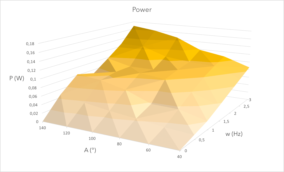
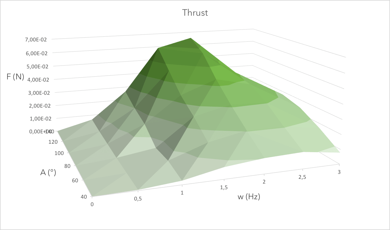
Study of the energetic consumption and the thrust force.
Introduction
Here we are going to analyse the thrust and the power needed for different couples (A,w). In this experiment we wrote an Arduino and a Python program that allow us to gather the information on the thrust force and the power at the same time.
Uncertainties
- Experimental : ∆O on the output given by the sensor and arduino circuit, also on the tension used to calculate the power,this time.
- Experimental : we checked after further examinations, that the amplitude of the fish was asymetrical. It generates more motion on one side of the fish than in the other side.
Protocol
- We turn on the alimentations of the fish and the force sensor.
- We set our fish on a certain couple (A,w).
-
We measure the force F on the sensor rod and the tension U at the servomotor’s terminals thanks to the Arduino circuit and program. We pay a special attention to the direction of the force captor since we learned in the previous experiment that it has a direction. Eventually with the relations below :
In an electric circuit, we have the following relations :
We have P the power delivered to a resistance, U the tension at its terminals and I the intensity. (NB : R = 1 Ohm)
P = U⋅I
U = R⋅I
The value of the tension is the value of the intensity by using the law of Ohm. The sensor can only measure tension from 0 to 5 volts. Therefore, we introduced a tension divider that got us the tension delivered to the fish divided by two. - We draw the curve of F in terms of (A,w) and P in terms of (A,w).
Constraints and Advantages
- For high frequencies: the fish will struggle to achieve high amplitudes, due to the limits of the servomotor. For instance, at 3Hz, the servomotor will not have time, in each oscillation, to access amplitudes higher than 60°.
- On the servomotor and the set-up: The servomotor doesn’t really deliver the exact amplitude A and frequency w that are set up in the Arduino’s program. Furthermore, due to a lack of time, we could not manage to fix the fish on the rod in a way that prevent any deformation during the experiment. Also, it will be hard to maintain a motion with high amplitude at high frequencies. This is the reason why we restrain the fish to a frequency range of [0.5Hz , 1Hz].
Results
Conclusion
POWER
THRUST