Compliant Swimming Robotic Fish

by Julien Bosse, Florian Terral and Joachim Mascaro


Introduction


  • Objective #1 : Deepen our knowledge domain

    Our field of study revolves around 4 fundamental domains of knowledge : rheology, hydrodynamics, torque and elasticity.

    Completing this project will not only give us the possibility to experiment the theory but also a chance to confirm if our methods are correct enough to do so.

    Therefore, we might learn how to validate the consistency of our results and how to experiment properly.

  • Objective #2: Improve the fish motion

    According to our supervisor, Professor Mederic Argentina, the caracteristic speed of our robotic fish U is proportionnal to A and w respectively the Amplitude of the tail (in degrees) and the Frequency (in Hertz) of its oscillation.

    U ~ Aw

    As a matter of fact, one can find different combinaison of (A,w) depending on the predation. For instance, a whale captures plankton with a high amplitude and a small frequency. On the opposite, a great white shark will hunt its prey by swimming with a medium amplitude and a high frequency.
  • Objective #3 : Energetic properties

    We are going to study the thrust force of our prototype and the power it consumes, and therefore we will investigate the energetic properties of our prototype.

    Each underwater species has its own way of locomotion. However, the speed U allows us to compare the efficiency and the properties of each motion.

    For instance, let's consider the case of the blue whale. It travels over hundreds of miles to feed on a microorganism called plankton, which is acknowledged to be static in seawater. Considering the distance of fishing and the poor amount of energy its prey provides, the whale must have a low energy consumption in order not to be starving after fishing.

    On the opposite, the killer whale energy optimization relies on a different logic. Orcas hunt a much faster prey - seals - and over shorter distances. Therefore, it must provide enough energy to reach the same speed U as their prey. The priority of the orca is not to save energy but to have enough speed to reach its prey whatever the amount of energy consumed.


gif

Calibration of the Hydraulic vein

The Hydraulic vein we use for our measures needs to be calibrated. Indeed, the only parameter we can change is the frequency at which the vein's motor runs. But in our future experiments, we will need to know the velocity of the flow. So to know what is the speed of the flow for different motor frequencies, we decided to calibrate the vein with the two following methods.

With the dye drop

Pic

colorant

Protocol in a nutshell :

  • Turn on the motor set on the frequency you desire to calibrate (between 8Hz and 50Hz), and wait a few instants for the flow to become stationnary.
  • Insert a drop of dye in the flow.
  • Wait for the dye to reach the field of the camera and launch the acquisition.
  • Process the data with ImageJ and use the formula V = d/t to obtain the speed V of the dye drop.

Result :

colorant

Conclusion:

The velocity of the flow inside the vein is linear. Therefore the theory is confirmed. However, the motor can provide frequencies up to 50Hz, but due to its limits, the relation between frequençy and flow velocity is not linear anymore for frequecies higher than 40Hz.

With the PIV

Pic

piv


Protocol in a nutshell :

  • Introduce particles with a small diameter (~µm) into the vein. Here, 20 µm diameter particles are used.
  • Turn on the motor and set it on the frequency you want to calibrate (between 8Hz and 50Hz).
  • Turn on the laser. Video acquisition is then processed on video software such as ImageJ and the data is treated to evaluate corrolation.
  • Extract data and convert it from “px/frame” to the format “cm/s”.

Result :

piv

Conclusion:

The experiment verifies the theory and according to it, the flow velocity is proportionnal to the frequency of the motor. The results with Particle Image Velocimetry are more precise than with the dye drop method, as you can see on the graphs.


Calibration of the force sensor

In order to have accurate measurements during our experiments, we need to calibrate the force sensor. The circuit gives us a tension U (in Volts), and we want a force F (in Newtons).

Pic

weigh

Protocol in a nutshell :

To calibrate our sensor, we are going to use objects (in this case bolts) with a certain mass (hence a certain weight). We decided to calibrate the sensor using the following method :
  • Weigh down the bolts with a scale to obtain their mass.
  • Calculate their weight in Newtons with the formula P = mg with g = 9.81 N/kg.
  • Using a string, hang a gobelet to the rod (force sensor mounted horizontally). Put the bolt(s) in it.
  • Measure the force it applies on the sensor when only subjected to gravity.
  • Gather all the data for each measure and then draw the curve of the force F in terms of the tension U.
  • The slope of the linear approximated curve will give us the conversion factor from the circuit output to the the real force applied on the force captor.

Result :

Here is the resulting curve of the tension U delivered by the force sensor and the circuit depending on the force F applied. This graph correspond to the rod #1. For example, in this case, F = (1/6.85)⋅U.

Conclusion:

We were succesfully able to calibrate a rod, we can now calibrate all of them and incorporate the recovered data.


capteur

Drag force


Disk

Drag force is defined by the following equation :

F = ½⋅pSCx


With :
  • p, the density of the fluid,
  • v, the speed of the object relative to the fluid,
  • S, the cross sectional,
  • Cx, the drag coefficient of the object.
In this experiment, we want to verify the theory by looking at the evolution of the force in terms of . To do so, we used a simple surface : a disk. We designed the solid with FreeCAD and Simplify3D and then 3D printed it.

Pic

piv

Protocol in a nutshell :

To determine the drag coefficient of the disk, we're going to measure its drag force against different flow velocities using the following method:
  • Place the disk on the sensor rod, making sure it faces the current.
  • Turn on the vein, starting at 10 Hz ( ≈ 3cm/s).
  • Proceed to the acquisition of the force thanks to the Arduino and Python programs.
  • Repeat this process with vein frequencies in [10Hz , 40Hz], with 5Hz-increments.

Result :

The result is a linear curve of F in terms of , which is exactly what we expected. And from the slope of this line, we can easily find the value of the disk drag coefficient using the formula of the drag force.

Conclusion:

We found Cx = 2,1 ± 0,1. We will use this value as comparison to the fish's drag coefficient.


disk

Drag coefficient of our fish

We then wanted to do the exact same experiment with our 3D-printed robotic fish (conception here). So we repeated the same procedure, replacing the disk with our fish. We obtained a similar relation between the drag force and . Thus we could calculate the drag coefficient of our fish :

Result:

We found Cx = 0.811 ± 0.019, wich is coherent with the value of the disk's Cx, since our fish is sleeker.


poisson

Tail's Movements

In this experiment, we will study the different movements of our fish, for a chosen (A,w) couple and acertain flow velocity. Indeed, the way the fish moves its tail can be chosen in a list of 5 different movements : Sin, Saw, Heavyside, Mix and Mix2.

Pic

Protocol in a nutshell :

  • Set up the fish and turn on the generators of the Arduino cricuit, force sensor and servomotor, along with the oscilloscope.
  • Choose a couple (A,w) and a flow velocity. For this experiment, we chose A = 90° and w = 1Hz using the Arduino program and set the vein's motor at 30 Hz. Then, using the Arduino program, choose the movement studied in the list : Sin, Saw, Heavyside, Mix or Mix2.
  • Launch the acquisition.
  • Draw the curve of the Angle (position of the tail) and the Force in terms of time.
  • Repeat this process for the 5 different movements.

Result :

You can see on the right the figures corresponding to the 5 different movements. There is the drag force applied on the fish by the current, and the position of the tail.

Conclusion:

We can see different patterns for the drag forces with the 5 different mouvements. So the type of mouvement and the way the fish moves its tail surely has an important impact on the drag force applied to the fish while he's swimming and facing a current.
-> For our future experiments, we decided to use the movement that looks like a fluid and realistic moving tail : the Sin.


mvmt

Velocity of the fish


Speed

This experiment leads us to the core of our project. Indeed, this is the part of the project which allows us to experiment over our supervisor's theory. In order to confirm this theory, we implemented the following experiment.

Protocol in a nutshell :

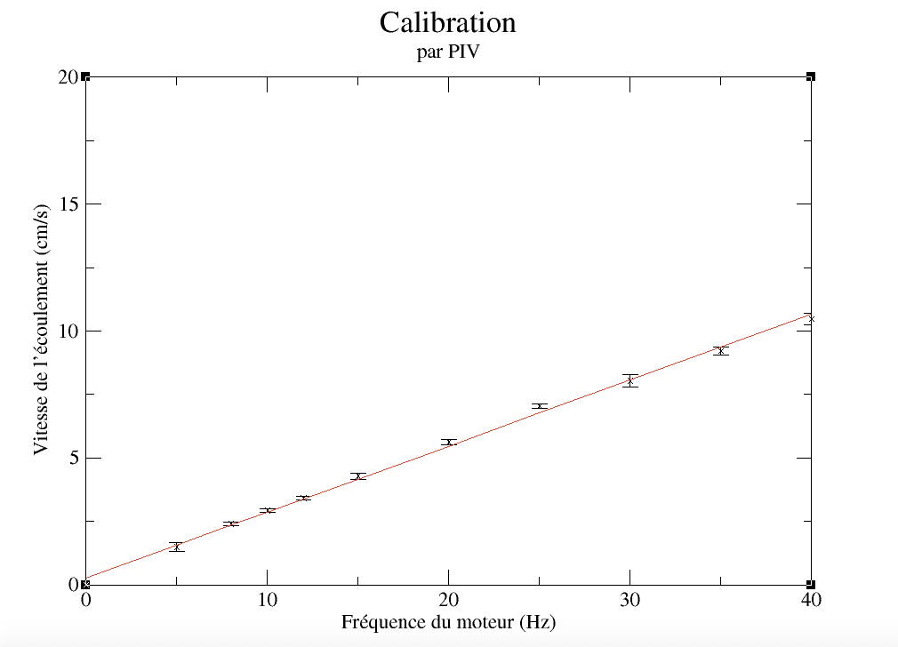
We decide to do this experiment at 6 different flow velocities (20Hz, 22.5Hz, 25Hz, 27.5Hz, 30Hz, 35Hz).
  • Measure the 0 (without speed from neither the vein nor the fish) for reference.
  • Switch on the vein at a given frequency corresponding to a certain stream velocity.
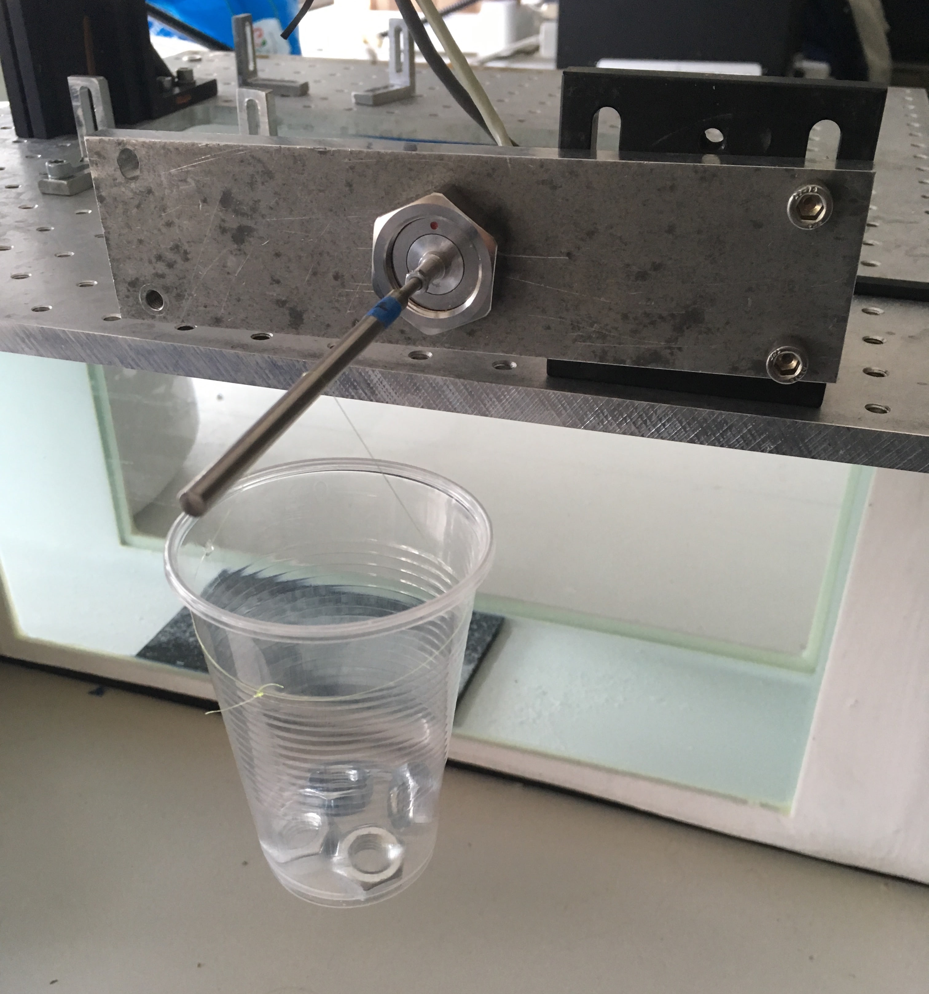
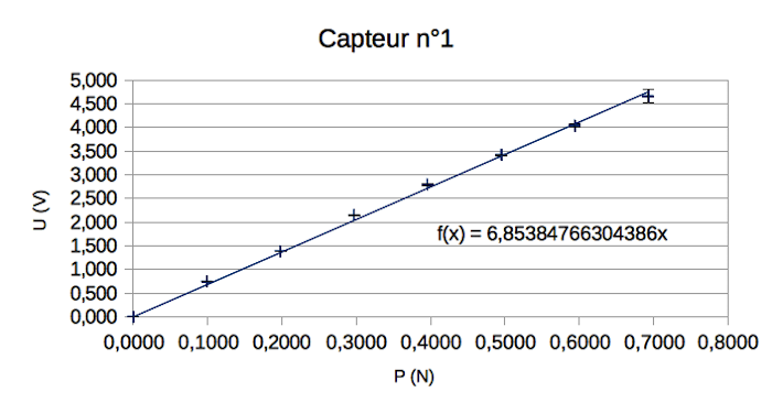
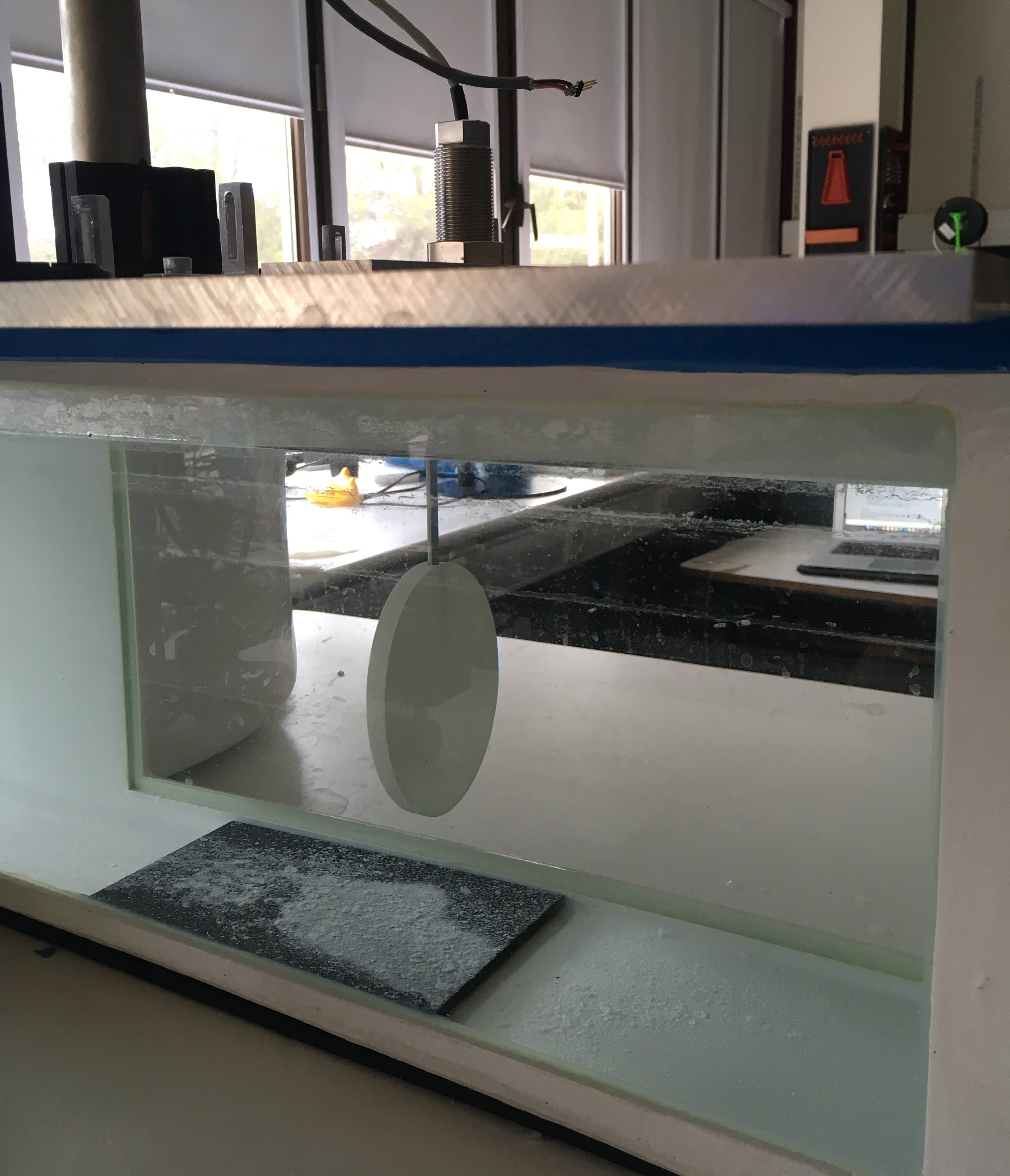
  • Begin an acquisition of the force measured by the force sensor, when the fish is moving at a certain couple (A,w).
  • Repeat the measure of the 0 before further measurements, since it changes between two measures.
  • Repeat for every couple (A,w) and then, repeat for each of the 6 different frequencies (flow velocities).

Result :

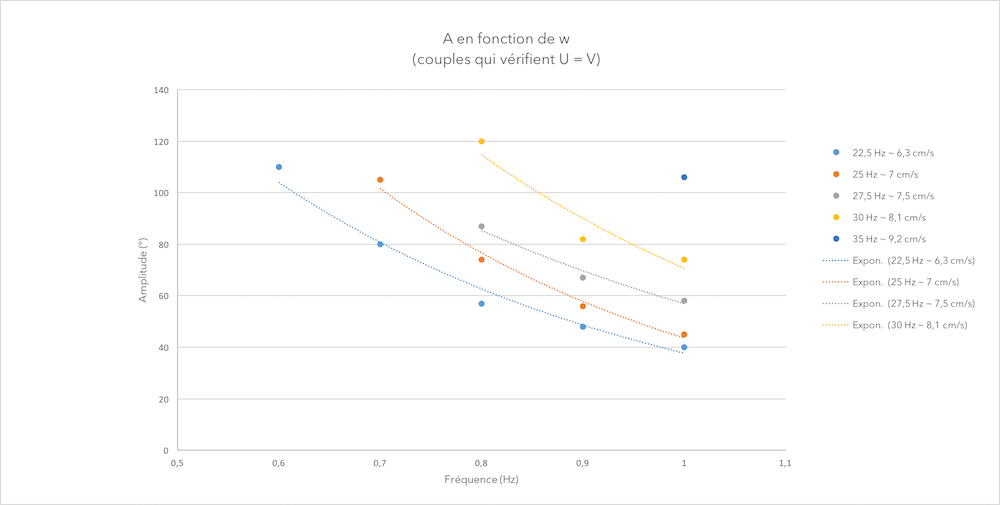
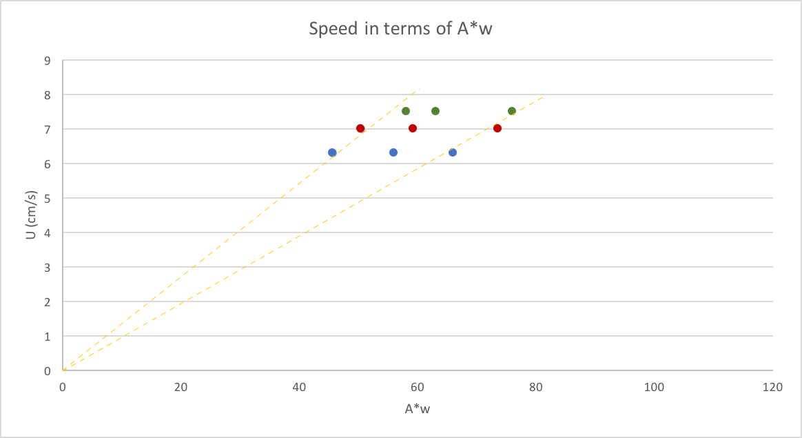
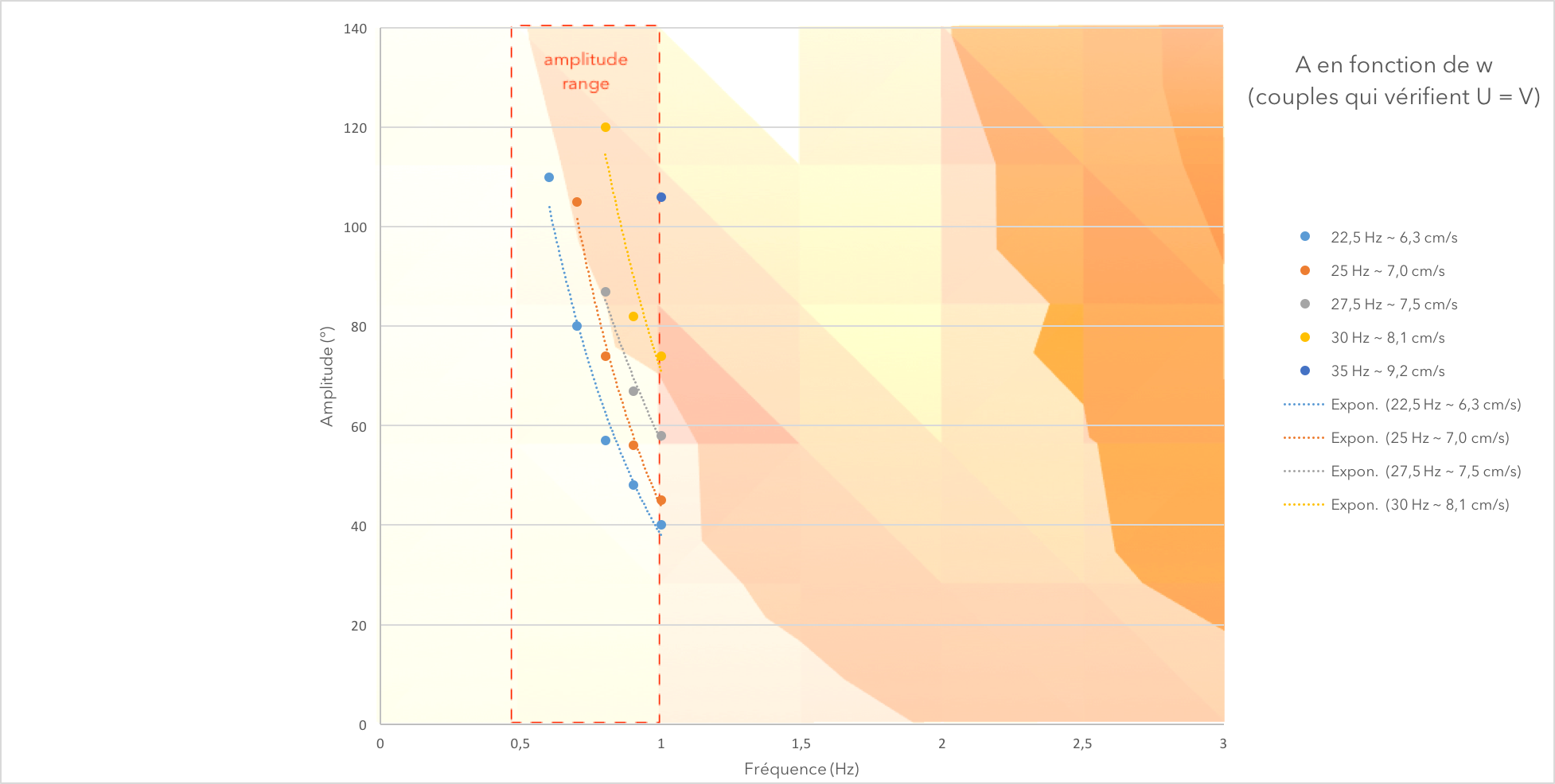
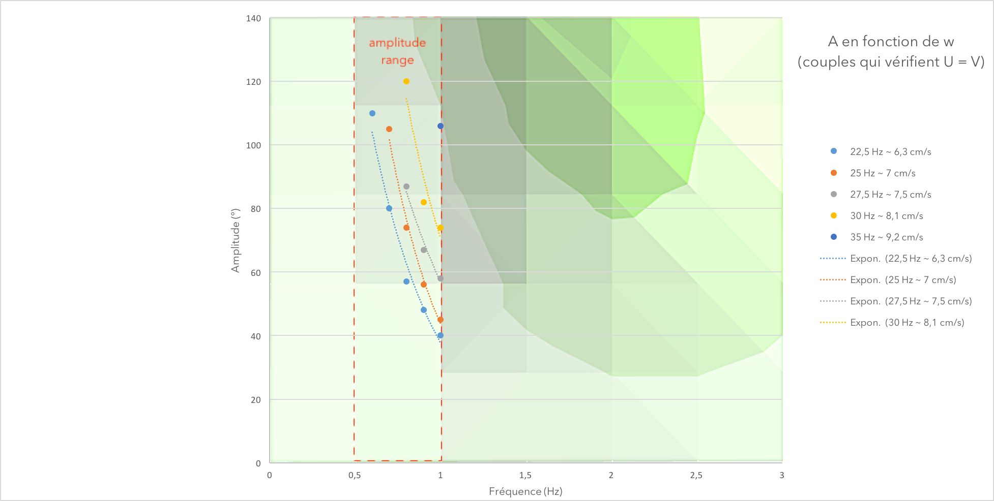
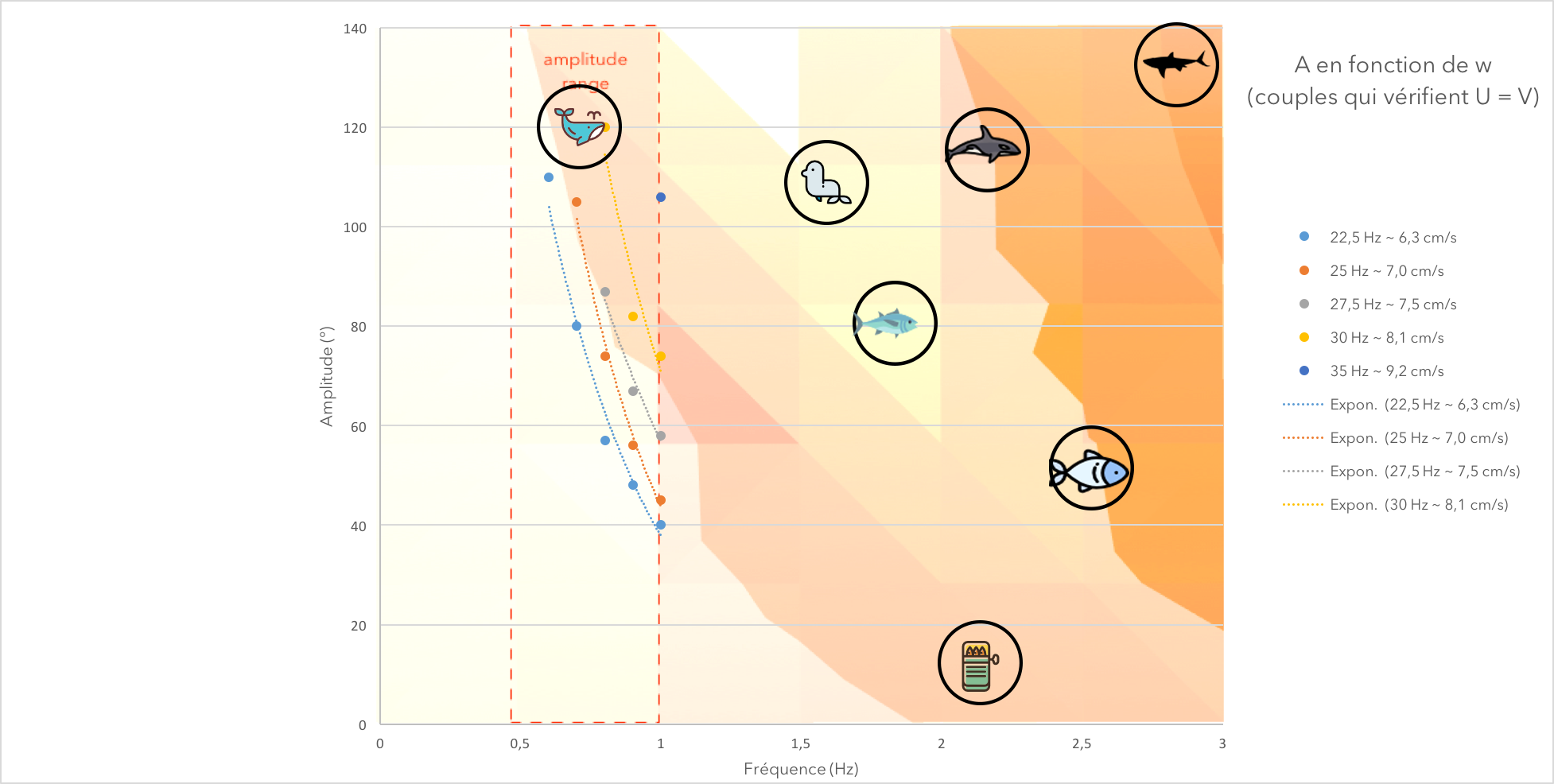
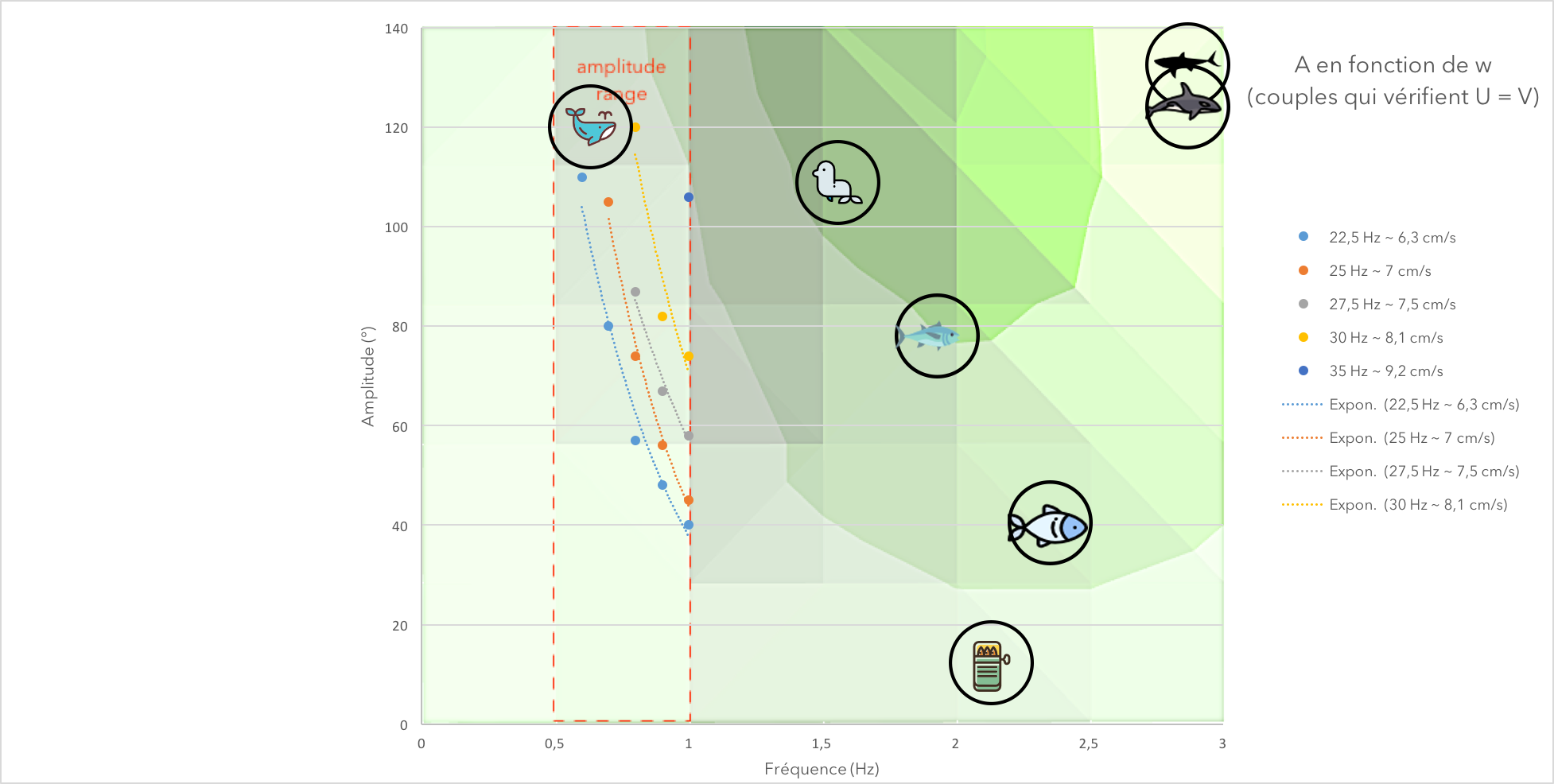
On the first figure, we can see 5 lines representing speed isolines. They are the set of couples (A,w) that verify a given speed. On the second one, we drew the speed in terms of each couple (A,w) under the form Aw (in the same color would be 3 couples that verify the same speed).

Conclusion:

With this experiment, we found different couples (A,w), verifying the same speed.
We now know exactly what couple of frequency and amplitude to apply if we want the fish to reach a certain speed. We also can see the possibilities an limits (lowest and highest speed) of our fish (due to the servomotor limits).
In addition to that, we can see on the second figure that the speed U of the fish depends linearly on the factor Aw, in accordance with Médéric Argentina's theory.


couples

couples

Thrust and Power


Here we are going to analyse the thrust and the power needed for different couples (A,w). In this experiment we wrote an Arduino and a Python program that allow us to gather the information on the thrust force and the power at the same time.

Protocol in a nutshell :

  • Turn on the alimentation of the fish and the force sensor.
  • Set our fish on a certain couple (A,w) using the Arduino program.
  • Measure the force F on the sensor rod and the tension U at the servomotor’s terminals thanks to the Arduino circuit and program. (We pay a special attention to the direction of the force captor since we learned in the previous experiment, it has a direction).
  • Draw the curve of F in terms of (A,w) and P in terms of (A,w).

Result :

As you can see on the right, we obtain 2 surfaces, representing the evolution of the Power needed by the servomotor (yellow) and the Thrust generated by the fish in movement (green) in terms of A (amplitude) and w (frequency) of the tail's movement.

Conclusion:

  • Power :
    As expected, the power needed by the servomotor to satisfy a certain couple (A,w) increases with the value of A and w. Indeed, logic dictates that the bigger A and w are, the bigger the energy needed is. The behaviour of the power provided is all the more logical since it is independent of whether the fish actually accomplishes the movement completely or not. The power only represents how many Watts the servomotor needs, but without the guarantee that it will be able to do it.

  • Thrust :
    We expected for the thrust to behave similarly as the power, but it appears it increases with the value of A and w only to a certain extent (up to certain value of the couple) which is (140°, 2Hz). We can conclude that this couple corresponds to the maximum thrust our fish can generate.
    This behaviour is caused by the fact that, at high frequencies, the tail cannot reach high amplitudes because of the servomotor limits.


thrust


power

End of the study

By looking at the speed analysis and the data provided by the energetic study, it is now possible to conclude on the project we started a couple of months ago.

Conclusion :


The previous graphic is the combination of the data provided by the study of the velocity and converted into a format that matches this Power chart, reduced in a 2D plan. Plus, we added the range of experimentation for the speed. This display of data provides some properties for the fish motion.

Indeed, the overview of the chart delivers a few properties :
  • The more movement our prototype produces, the more energy it consumes. There are obviously three areas we can interpret as three levels of energy consumption : low, medium and high.
  • Besides, the curves of iso-velocity appears to be parallel to the curves that delimitates the previous area of energy.
  • This also means that one level of energy can have different solutions in terms of couples (A,w).

In the previous chart, drawn on the same basis as the first one, it is possible to discern a few aspects about the conditions of the project:
  • The more an animal provides motion, the more powerful its thrust should be.
  • The theory is partly unverifiable due to the conditions of experimentation.
  • In fact, the peak marked in bright green should be on the right corner.
  • It is possible for an animal to provide the same thrust by using different combinaisons of A and w.


Opening:


If we place the different motions on the previous graphics, we would be able to check the theory.

Even if the measurements of each animal tail are empirical, it is still possible to have an idea about the energetic consumption and the thrust force provided by the tail.

Indeed, this display allows us to confirm our results. The power charts seems to be physically correct because of plausibleness of the motion for different animals.

Therefore, a certain level of energy can be delivered in different combinaisons of (A,w). Each of them matches the predation type of each amphibious.

Of course, it is possible for each species to change its level of energy.


On the opposite, the thrust chart doesn’t seem acceptable since the top strength could be reached by animals such as seals and tuna. Therefore, the reader would easily remark the existence of a mistake.

This mistake comes from the making of the prototype itself.

During the experimentation, we observed that the robot rotates around the rod it was fixed on. Therefore, the measurements are not accurate for high frequencies and a part of the strength provided by the tail is dissipated in the rotation. Also, the amplitude of the motion of the tail was asymetric – leaving the fish moving its tail more on its right flank than on its left one.