The new chaotic pendulum

Preliminary study
case of the simple pendulum

We will begin the study of our pendulum by the most simple case we can encounter: the simple pendulum. It is in fact only constituted of a weight $m$, oscillating without friction in a plane, and suspended by a string of length $l$ and with no mass. This system is subjected to the gravity $\vec{g}$.

Positions and speeds

Let us begin by seeking the coordinates of the weight regarding the angle $\theta$, and the corresponding speeds: $$ \left \{ \begin{array}{r c l} x & = & l \sin \theta \\ y & = & 0 \\ z & = & -l \cos \theta \\ \end{array} \right . \; \Rightarrow \; \left \{ \begin{array}{r c l} \dot{x} & = & l \dot{\theta} \cos \theta \\ \dot{z} & = & l \dot{\theta}\sin \theta\\ \end{array} \right . $$

Energies, Lagrangian and movement equation

We can then find the kinetic and potential energy, and thus the corresponding Lagrangian ^[ref] $\mathcal{L}$:
$$ \left . \begin{array}{r c l} E_k & = & \frac{1}{2}mv^2=\frac{1}{2}m\left(\sqrt{\dot{x}^2+\dot{y}^2+\dot{z}^2}\right)^2 \\ & = & \frac{1}{2}ml^2\dot{\theta}^2\\ \\ E_p & = & -\vec{W}\cdot\vec{r}=mgz=-mgl\cos\theta\\ \\ \\ L & = & E_k-E_p\\ & = & \frac{1}{2}ml^2\dot{\theta}^2+mgl\cos\theta\\ \end{array} \right . $$

The Euler-Lagrange equations give us, with $\theta$ as a generalized coordinate: $$ \begin{eqnarray} \frac{\partial L}{\partial \theta} = \frac{\text{d}}{\text{d}t}\frac{\partial L}{\partial\dot{\theta}} \; & \Rightarrow \; & \ddot{\theta}=-\frac{g}{l}\sin\theta \end{eqnarray} $$

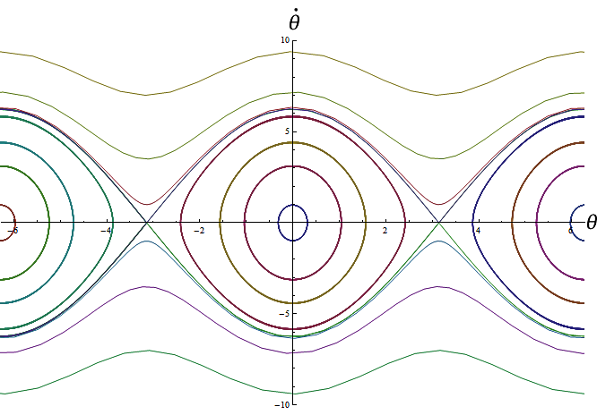
Trajectory and phase diagram

We will now integrate the equation above to get the simple pendulum's spatial trajectory and phase diagram.
Since the movement is made in a plan, it is easy to guess that the trajectory will be a part of a circle. On va maintenant intégrer l'équation obtenue pour obtenir la trajectoire spatiale et le portrait de phase du pendule simple.
Le mouvement étant plan, la trajectoire est aisée à deviner: on obtiendra une portion de cercle.