The new chaotic pendulum

Preliminary study
case of the spherical pendulum

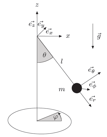
We will now study the case of the spherical pendulum. We add another degree of freedom to the case of the simple pendulum : the mass can now rotate around the $z$ axis, doing an angle $\varphi$ with the $x$ axis. The movement will now be tri-dimensionnal.

Positions and speeds

We begin by seeking the mass' coordinates and corresponding speeds, with respect to the angles $\theta$ and $\varphi$ : $$ \left \{ \begin{array}{r c l} x & = & l \sin \theta \cos \varphi \\ y & = & l \sin \theta \sin \varphi \\ z & = & -l \cos \theta \end{array} \right . \; \Rightarrow \; \left \{ \begin{array}{r c l} \dot{x} & = & l (\dot{\theta} \cos \theta \cos \varphi - \dot{\varphi} \sin \theta \sin \varphi ) \\ \dot{y} & = & l (\dot{\theta} \cos \theta \sin \varphi + \dot{\varphi} \sin \theta \cos \varphi )\\ \dot{z} & = & l \dot{\theta} \sin \theta \end{array} \right . $$

energies, Lagrangian, movement equations

We may then find the potential and kinetic energies, and thus the corresponding Lagrangian $\mathcal{L}$ :
$$ \begin{eqnarray*} E_k & = & \frac{1}{2}m v^2=\frac{m}{2}(\dot{x}^2+\dot{y}^2+\dot{z}^2)=\frac{m l^2}{2}(\dot{\theta}^2+\dot{\varphi}^2\sin^2\theta) \\ E_p & = & -\vec{P}\cdot\vec{r}=mgz=-mgl\cos\theta \\ \\ \mathcal{L} & = & E_k - E_p = \frac{m l^2}{2}(\dot{\theta}^2+\dot{\varphi}^2\sin^2\theta) + mgl\cos\theta \end{eqnarray*}\\ $$ From this we deduce the Euler-Lagrange equations : $$ \begin{eqnarray} \frac{\partial \mathcal{L}}{\partial \theta} = \frac{\text{d}}{\text{d} t}\frac{\partial \mathcal{L}}{\partial\dot{\theta}} \; & \Rightarrow \; & \ddot{\theta}=\dot{\varphi}^2\sin\theta\cos\theta-\frac{g}{l}\sin\theta \\ % \frac{\partial \mathcal{L}}{\partial \varphi} = \frac{\text{d}}{\text{d} t}\frac{\partial \mathcal{L}}{\partial\dot{\varphi}} \; & \Rightarrow \; & \ddot{\varphi}=-2\dot{\theta}\dot{\varphi}\cot\theta \end{eqnarray} $$

Integrating the equations

We can now integrate numerically the new-found coupled equations (we will use here Wolfram Mathematica 8 ).
Finally, we get the following trajectories, which of course depend of the initial conditions we chose :

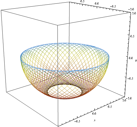
We can notice that the central area is never reached by the pendulum, and the "bowl"-shaped trajectories : the pendulum now describes a part of a sphere.
Like for the case of the simple pendulum, the mechanic energy is conserved, and the kinetic energy $E_k$ becomes zero for a same value of the potential enery $E_p$ – the pendulum then reaches a maximal height and "falls" again.